Measuring the speed of an algorithm in real time—in seconds and minutes—is not easy. One program may run slower than another not because of its own inefficiency, but because of the slowness of the operating system, incompatibility with hardware, computer memory being occupied by other processes... To measure the effectiveness of algorithms, universal concepts have been invented, regardless of the environment in which the program is running. The asymptotic complexity of a problem is measured using Big O notation. Let f(x) and g(x) be functions defined in a certain neighborhood of x0, and g does not vanish there. Then f is “O” greater than g for (x -> x0) if there is a constant C>0 , that for all x from some neighborhood of the point x0 the inequality holds. |f(x)| <= C |g(x)| Slightly less strict: f is “O” greater than g if there is a constant C>0, which for all x > x0 f(x) <= C*g(x) Don’t be afraid of the formal definition! Essentially, it determines the asymptotic increase in program running time when the amount of your input data grows towards infinity. For example, you are comparing sorting an array of 1000 elements and 10 elements, and you need to understand how the program’s running time will increase. Or you need to calculate the length of a string of characters by going character by character and adding 1 for each character: c - 1 a - 2 t - 3 Its asymptotic speed = O(n), where n is the number of letters in the word. If you count according to this principle, the time required to count the entire line is proportional to the number of characters. Counting the number of characters in a 20-character string takes twice as long as counting the number of characters in a ten-character string. Imagine that in the length variable you stored a value equal to the number of characters in the string. For example, length = 1000. To get the length of a string, you only need access to this variable; you don’t even have to look at the string itself. And no matter how we change the length, we can always access this variable. In this case, asymptotic speed = O(1). Changing the input data does not change the speed of such a task; the search is completed in a constant time. In this case, the program is asymptotically constant. Disadvantage: You waste computer memory storing an additional variable and additional time updating its value. If you think that linear time is bad, we can assure you that it can be much worse. For example, O(n 2 ). This notation means that as n grows, the time required to iterate through elements (or another action) will grow more and more sharply. But for small n, algorithms with asymptotic speed O(n 2 ) can work faster than algorithms with asymptotic speed O(n). But at some point the quadratic function will overtake the linear one, there is no way around it. Another asymptotic complexity is logarithmic time or O(log n). As n increases, this function increases very slowly. O(log n) is the running time of the classic binary search algorithm in a sorted array (remember the torn telephone directory in the lecture?). The array is divided in two, then the half in which the element is located is selected, and so, each time reducing the search area by half, we search for the element. What happens if we immediately stumble upon what we are looking for, dividing our data array in half for the first time? There is a term for the best time - Omega-large or Ω(n). In the case of binary search = Ω(1) (finds in constant time, regardless of the size of the array). Linear search runs in O(n) and Ω(1) time if the element being searched is the very first one. Another symbol is theta (Θ(n)). It is used when the best and worst options are the same. This is suitable for an example where we stored the length of a string in a separate variable, so for any length it is enough to refer to this variable. For this algorithm, the best and worst cases are Ω(1) and O(1), respectively. This means that the algorithm runs in time Θ(1).
Linear search
When you open a web browser, look for a page, information, friends on social networks, you are doing a search, just like when trying to find the right pair of shoes in a store. You've probably noticed that orderliness has a big impact on how you search. If you have all your shirts in your closet, it is usually easier to find the one you need among them than among those scattered without a system throughout the room. Linear search is a method of sequential search, one by one. When you review Google search results from top to bottom, you are using a linear search. Example . Let's say we have a list of numbers: 2 4 0 5 3 7 8 1 And we need to find 0. We see it right away, but a computer program doesn't work that way. She starts at the beginning of the list and sees the number 2. Then she checks, 2=0? It's not, so she continues and moves on to the second character. Failure awaits her there too, and only in the third position does the algorithm find the required number. Pseudo-code for linear search: The linearSearch function receives two arguments as input - the key key and the array array[]. The key is the desired value, in the previous example key = 0. The array is a list of numbers that we will look through. If we didn't find anything, the function will return -1 (a position that doesn't exist in the array). If the linear search finds the desired element, the function will return the position at which the desired element is located in the array. The good thing about linear search is that it will work for any array, regardless of the order of the elements: we will still go through the entire array. This is also his weakness. If you need to find the number 198 in an array of 200 numbers sorted in order, the for loop will go through 198 steps. You've probably already guessed which method works better for a sorted array?
Binary search and trees
Imagine you have a list of Disney characters sorted alphabetically and you need to find Mickey Mouse. Linearly it would take a long time. And if we use the “method of tearing the directory in half,” we get straight to Jasmine, and we can safely discard the first half of the list, realizing that Mickey cannot be there. Using the same principle, we discard the second column. Continuing this strategy, we will find Mickey in just a couple of steps. Let's find the number 144. We divide the list in half, and we get to the number 13. We evaluate whether the number we are looking for is greater or less than 13. 13 < 144, so we can ignore everything to the left of 13 and this number itself. Now our search list looks like this: There is an even number of elements, so we choose the principle by which we select the “middle” (closer to the beginning or end). Let's say we chose the strategy of proximity to the beginning. In this case, our "middle" = 55. 55 < 144. We discard the left half of the list again. Luckily for us, the next average number is 144. We found 144 in a 13-element array using binary search in just three steps. A linear search would handle the same situation in as many as 12 steps. Since this algorithm reduces the number of elements in the array by half at each step, it will find the required one in asymptotic time O(log n), where n is the number of elements in the list. That is, in our case, the asymptotic time = O(log 13) (this is a little more than three). Pseudocode of the binary search function: The function takes 4 arguments as input: the desired key, the data array array [], in which the desired one is located, min and max are pointers to the maximum and minimum number in the array, which we are looking at at this step of the algorithm. For our example, the following picture was initially given: Let’s analyze the code further. midpoint is our middle of the array. It depends on the extreme points and is centered between them. After we have found the middle, we check if it is less than our key number. If so, then key is also greater than any of the numbers to the left of the middle, and we can call the binary function again, only now our min = midpoint + 1. If it turns out that key < midpoint, we can discard that number itself and all the numbers , lying to his right. And we call a binary search through the array from the number min and up to the value (midpoint – 1). Finally, the third branch: if the value in midpoint is neither greater nor less than key, it has no choice but to be the desired number. In this case, we return it and finish the program. Finally, it may happen that the number you are looking for is not in the array at all. To take this case into account, we perform the following check: And we return (-1) to indicate that we didn't find anything. You already know that binary search requires the array to be sorted. Thus, if we have an unsorted array in which we need to find a certain element, we have two options:
Sort the list and apply binary search
Keep the list always sorted while simultaneously adding and removing elements from it.
One way to keep lists sorted is to use a binary search tree. A binary search tree is a data structure that meets the following requirements:
It is a tree (a data structure that emulates a tree structure - it has a root and other nodes (leaves) connected by “branches” or edges without cycles)
Each node has 0, 1 or 2 children
Both left and right subtrees are binary search trees.
All nodes of the left subtree of an arbitrary node X have data key values less than the value of the data key of node X itself.
All nodes in the right subtree of an arbitrary node X have data key values greater than or equal to the value of the data key of node X itself.
Attention: the root of the “programmer” tree, unlike the real one, is at the top. Each cell is called a vertex, and the vertices are connected by edges. The root of the tree is cell number 13. The left subtree of vertex 3 is highlighted in color in the picture below: Our tree meets all the requirements for binary trees. This means that each of its left subtrees contains only values that are less than or equal to the value of the vertex, while the right subtree contains only values greater than or equal to the value of the vertex. Both left and right subtrees are themselves binary subtrees. The method of constructing a binary tree is not the only one: below in the picture you see another option for the same set of numbers, and there can be a lot of them in practice. This structure helps to carry out the search: we find the minimum value by moving from the top to the left and down each time. If you need to find the maximum number, we go from the top down and to the right. Finding a number that is not the minimum or maximum is also quite simple. We descend from the root to the left or to the right, depending on whether our vertex is larger or smaller than the one we are looking for. So, if we need to find the number 89, we go through this path: You can also display the numbers in sorting order. For example, if we need to display all the numbers in ascending order, we take the left subtree and, starting from the leftmost vertex, go up. Adding something to the tree is also easy. The main thing to remember is the structure. Let's say we need to add the value 7 to the tree. Let's go to the root and check. The number 7 < 13, so we go left. We see 5 there, and we go to the right, since 7 > 5. Further, since 7 > 8 and 8 has no descendants, we construct a branch from 8 to the left and attach 7 to it. You can also remove vertices from the tree, but this is somewhat more complicated. There are three different deletion scenarios that we need to consider.
The simplest option: we need to delete a vertex that has no children. For example, the number 7 we just added. In this case, we simply follow the path to the vertex with this number and delete it.
A vertex has one child vertex. In this case, you can delete the desired vertex, but its descendant must be connected to the “grandfather”, that is, the vertex from which its immediate ancestor grew. For example, from the same tree we need to remove the number 3. In this case, we join its descendant, one, together with the entire subtree to 5. This is done simply, since all the vertices to the left of 5 will be less than this number (and less than remote triple).
The most difficult case is when the vertex being deleted has two children. Now the first thing we need to do is find the vertex in which the next larger value is hidden, we need to swap them, and then delete the desired vertex. Note that the next highest value vertex cannot have two children, then its left child will be the best candidate for the next value. Let's remove the root node 13 from our tree. First, we look for the number closest to 13, which is greater than it. This is 21. Swap 21 and 13 and delete 13.
There are different ways to build binary trees, some good, others not so good. What happens if we try to build a binary tree from a sorted list? All numbers will simply be added to the right branch of the previous one. If we want to find a number, we will have no choice but to simply follow the chain down. It's no better than linear search. There are other data structures that are more complex. But we won’t consider them for now. Let's just say that to solve the problem of constructing a tree from a sorted list, you can randomly mix the input data.
Sorting algorithms
There is an array of numbers. We need to sort it. For simplicity, we will assume that we are sorting the integers in ascending order (from smallest to largest). There are several known ways to accomplish this process. Plus, you can always dream up the topic and come up with a modification of the algorithm.
Sorting by selection
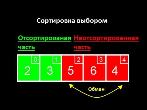
The main idea is to split our list into two parts, sorted and unsorted. At each step of the algorithm, a new number is moved from the unsorted part to the sorted part, and so on until all the numbers are in the sorted part.
Find the minimum unsorted value.
We swap this value with the first unsorted value, thus placing it at the end of the sorted array.
If there are unsorted values left, return to step 1.
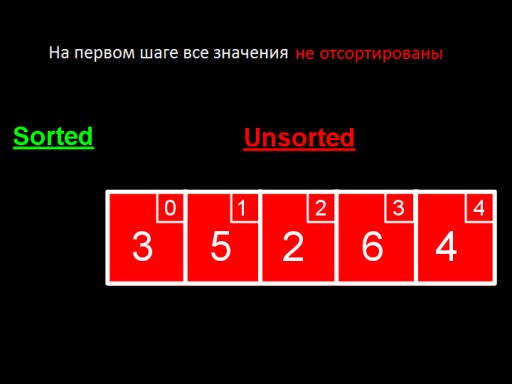
In the first step, all values are unsorted. Let's call the unsorted part Unsorted, and the sorted part Sorted (these are just English words, and we do this only because Sorted is much shorter than “Sorted part” and will look better in pictures). We find the minimum number in the unsorted part of the array (that is, at this step - in the entire array). This number is 2. Now we change it with the first among the unsorted ones and put it at the end of the sorted array (at this step - in first place). In this step, this is the first number in the array, that is, 3. Step two. We don’t look at the number 2; it’s already in the sorted subarray. We start looking for the minimum, starting from the second element, this is 5. We make sure that 3 is the minimum among the unsorted, 5 is the first among the unsorted. We swap them and add 3 to the sorted subarray. In the third step , we see that the smallest number in the unsorted subarray is 4. We change it with the first number among the unsorted ones - 5. In the fourth step, we find that in the unsorted array the smallest number is 5. We change it from 6 and add it to the sorted subarray . When only one number remains among the unsorted ones (the largest), this means that the entire array is sorted! This is what the array implementation looks like in code. Try making it yourself. In both the best and worst cases, to find the minimum unsorted element, we must compare each element with each element of the unsorted array, and we will do this at each iteration. But we do not need to view the entire list, but only the unsorted part. Does this change the speed of the algorithm? In the first step, for an array of 5 elements, we make 4 comparisons, in the second - 3, in the third - 2. To get the number of comparisons, we need to add up all these numbers. We get the sum Thus, the expected speed of the algorithm in the best and worst cases is Θ(n 2 ). Not the most efficient algorithm! However, for educational purposes and for small data sets it is quite applicable.
Bubble sort
The bubble sort algorithm is one of the simplest. We go along the entire array and compare 2 neighboring elements. If they are in the wrong order, we swap them. On the first pass, the smallest element will appear (“float”) at the end (if we sort in descending order). Repeat the first step if at least one exchange was completed in the previous step. Let's sort the array. Step 1: go through the array. The algorithm starts with the first two elements, 8 and 6, and checks to see if they are in the correct order. 8 > 6, so we swap them. Next we look at the second and third elements, now these are 8 and 4. For the same reasons, we swap them. For the third time we compare 8 and 2. In total, we make three exchanges (8, 6), (8, 4), (8, 2). The value 8 "floated" to the end of the list in the correct position. Step 2: swap (6,4) and (6,2). 6 is now in the penultimate position, and there is no need to compare it with the already sorted “tail” of the list. Step 3: swap 4 and 2. The four “floats up” to its rightful place. Step 4: we go through the array, but we have nothing to change. This signals that the array is completely sorted. And this is the algorithm code. Try implementing it in C! Bubble sort takes O(n 2 ) time in the worst case (all numbers are wrong), since we need to take n steps at each iteration, of which there are also n. In fact, as in the case of the selection sort algorithm, the time will be slightly less (n 2 /2 – n/2), but this can be neglected. In the best case (if all the elements are already in place), we can do it in n steps, i.e. Ω(n), since we will just need to iterate through the array once and make sure that all the elements are in place (i.e. even n-1 elements).
Insertion sort
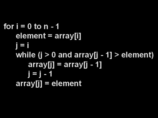
The main idea of this algorithm is to divide our array into two parts, sorted and unsorted. At each step of the algorithm, the number moves from the unsorted to the sorted part. Let's look at how insertion sort works using the example below. Before we start, all elements are considered unsorted. Step 1: Take the first unsorted value (3) and insert it into the sorted subarray. At this step, the entire sorted subarray, its beginning and end will be this very three. Step 2: Since 3 > 5, we will insert 5 into the sorted subarray to the right of 3. Step 3: Now we work on inserting the number 2 into our sorted array. We compare 2 with values from right to left to find the correct position. Since 2 < 5 and 2 < 3 and we have reached the beginning of the sorted subarray. Therefore, we must insert 2 to the left of 3. To do this, move 3 and 5 to the right so that there is room for the 2 and insert it at the beginning of the array. Step 4. We're lucky: 6 > 5, so we can insert that number right after the number 5. Step 5. 4 < 6 and 4 < 5, but 4 > 3. Therefore, we know that 4 must be inserted to the right of 3. Again, we are forced to move 5 and 6 to the right to create a gap for 4. Done! Generalized Algorithm: Take each unsorted element of n and compare it with the values in the sorted subarray from right to left until we find a suitable position for n (that is, the moment we find the first number that is less than n). Then we shift all the sorted elements that are to the right of this number to the right to make room for our n, and we insert it there, thereby expanding the sorted part of the array. For each unsorted element n you need:
Determine the location in the sorted part of the array where n should be inserted
Shift sorted elements to the right to create a gap for n
Insert n into the resulting gap in the sorted part of the array.
And here is the code! We recommend writing your own version of the sorting program.
Asymptotic speed of the algorithm
In the worst case, we will make one comparison with the second element, two comparisons with the third, and so on. Thus our speed is O(n 2 ). At best, we will be working with an already sorted array. The sorted part, which we build from left to right without insertions and movements of elements, will take time Ω(n).
Merge sort
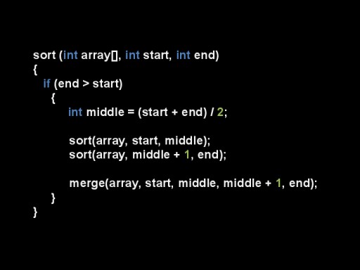
This algorithm is recursive; it breaks one large sorting problem into subtasks, the execution of which makes it closer to solving the original large problem. The main idea is to split an unsorted array into two parts and sort the individual halves recursively. Let's say we have n elements to sort. If n < 2, we finish sorting, otherwise we sort the left and right parts of the array separately, and then combine them. Let's sort the array. Divide it into two parts, and continue dividing until we get subarrays of size 1, which are obviously sorted. Two sorted subarrays can be merged in O(n) time using a simple algorithm: remove the smaller number at the beginning of each subarray and insert it into the merged array. Repeat until all the elements are gone. Merge sort takes O(nlog n) time for all cases. While we are dividing the arrays into halves at each recursion level we get log n. Then, merging the subarrays requires only n comparisons. Therefore O(nlog n). The best and worst cases for merge sort are the same, the expected running time of the algorithm = Θ(nlog n). This algorithm is the most effective among those considered.
 But at some point the quadratic function will overtake the linear one, there is no way around it. Another asymptotic complexity is logarithmic time or O(log n). As n increases, this function increases very slowly. O(log n) is the running time of the classic binary search algorithm in a sorted array (remember the torn telephone directory in the lecture?). The array is divided in two, then the half in which the element is located is selected, and so, each time reducing the search area by half, we search for the element.
  What happens if we immediately stumble upon what we are looking for, dividing our data array in half for the first time? There is a term for the best time - Omega-large or Ω(n). In the case of binary search = Ω(1) (finds in constant time, regardless of the size of the array). Linear search runs in O(n) and Ω(1) time if the element being searched is the very first one. Another symbol is theta (Θ(n)). It is used when the best and worst options are the same. This is suitable for an example where we stored the length of a string in a separate variable, so for any length it is enough to refer to this variable. For this algorithm, the best and worst cases are Ω(1) and O(1), respectively. This means that the algorithm runs in time Θ(1).
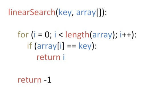 linearSearch function receives two arguments as input - the key key and the array array[]. The key is the desired value, in the previous example key = 0. The array is a list of numbers that we will look through. If we didn't find anything, the function will return -1 (a position that doesn't exist in the array). If the linear search finds the desired element, the function will return the position at which the desired element is located in the array. The good thing about linear search is that it will work for any array, regardless of the order of the elements: we will still go through the entire array. This is also his weakness. If you need to find the number 198 in an array of 200 numbers sorted in order, the for loop will go through 198 steps.
  You've probably already guessed which method works better for a sorted array?

 Linearly it would take a long time. And if we use the “method of tearing the directory in half,” we get straight to Jasmine, and we can safely discard the first half of the list, realizing that Mickey cannot be there.
  Using the same principle, we discard the second column. Continuing this strategy, we will find Mickey in just a couple of steps.
  Let's find the number 144. We divide the list in half, and we get to the number 13. We evaluate whether the number we are looking for is greater or less than 13. 13
  < 144, so we can ignore everything to the left of 13 and this number itself. Now our search list looks like this:
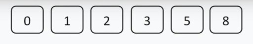
 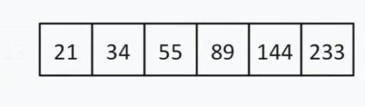 There is an even number of elements, so we choose the principle by which we select the “middle” (closer to the beginning or end). Let's say we chose the strategy of proximity to the beginning. In this case, our "middle" = 55.
  55 < 144. We discard the left half of the list again. Luckily for us, the next average number is 144.
  We found 144 in a 13-element array using binary search in just three steps. A linear search would handle the same situation in as many as 12 steps. Since this algorithm reduces the number of elements in the array by half at each step, it will find the required one in asymptotic time O(log n), where n is the number of elements in the list. That is, in our case, the asymptotic time = O(log 13) (this is a little more than three). Pseudocode of the binary search function:
 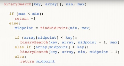 The function takes 4 arguments as input: the desired key, the data array array [], in which the desired one is located, min and max are pointers to the maximum and minimum number in the array, which we are looking at at this step of the algorithm. For our example, the following picture was initially given:
  Let’s analyze the code further. midpoint is our middle of the array. It depends on the extreme points and is centered between them. After we have found the middle, we check if it is less than our key number.
  If so, then key is also greater than any of the numbers to the left of the middle, and we can call the binary function again, only now our min = midpoint + 1. If it turns out that key < midpoint, we can discard that number itself and all the numbers , lying to his right. And we call a binary search through the array from the number min and up to the value (midpoint – 1).
  Finally, the third branch: if the value in midpoint is neither greater nor less than key, it has no choice but to be the desired number. In this case, we return it and finish the program.
  Finally, it may happen that the number you are looking for is not in the array at all. To take this case into account, we perform the following check:
  And we return (-1) to indicate that we didn't find anything. You already know that binary search requires the array to be sorted. Thus, if we have an unsorted array in which we need to find a certain element, we have two options:
 Attention: the root of the “programmer” tree, unlike the real one, is at the top. Each cell is called a vertex, and the vertices are connected by edges. The root of the tree is cell number 13. The left subtree of vertex 3 is highlighted in color in the picture below:
 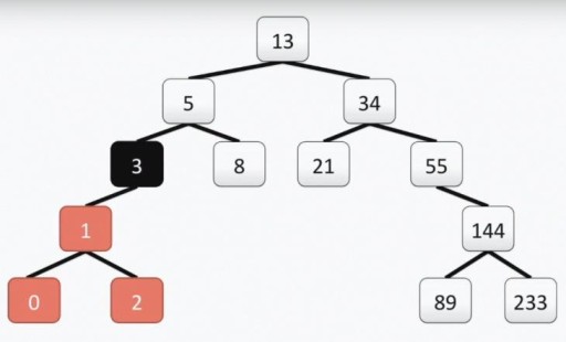 Our tree meets all the requirements for binary trees. This means that each of its left subtrees contains only values that are less than or equal to the value of the vertex, while the right subtree contains only values greater than or equal to the value of the vertex. Both left and right subtrees are themselves binary subtrees. The method of constructing a binary tree is not the only one: below in the picture you see another option for the same set of numbers, and there can be a lot of them in practice.
  This structure helps to carry out the search: we find the minimum value by moving from the top to the left and down each time.
 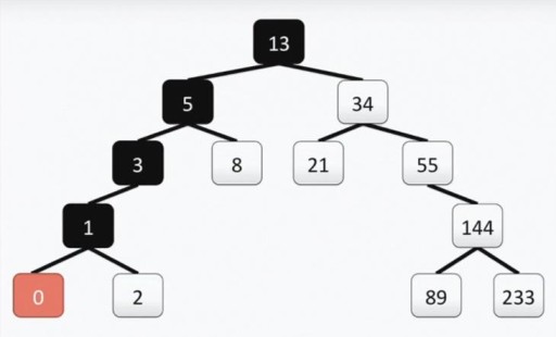 If you need to find the maximum number, we go from the top down and to the right. Finding a number that is not the minimum or maximum is also quite simple. We descend from the root to the left or to the right, depending on whether our vertex is larger or smaller than the one we are looking for. So, if we need to find the number 89, we go through this path:
  You can also display the numbers in sorting order. For example, if we need to display all the numbers in ascending order, we take the left subtree and, starting from the leftmost vertex, go up. Adding something to the tree is also easy. The main thing to remember is the structure. Let's say we need to add the value 7 to the tree. Let's go to the root and check. The number 7 < 13, so we go left. We see 5 there, and we go to the right, since 7 > 5. Further, since 7 > 8 and 8 has no descendants, we construct a branch from 8 to the left and attach 7 to it. You can also remove
 vertices from the tree, but this is somewhat more complicated. There are three different deletion scenarios that we need to consider.


 All numbers will simply be added to the right branch of the previous one. If we want to find a number, we will have no choice but to simply follow the chain down.
  It's no better than linear search. There are other data structures that are more complex. But we won’t consider them for now. Let's just say that to solve the problem of constructing a tree from a sorted list, you can randomly mix the input data.
 The main idea is to split our list into two parts, sorted and unsorted. At each step of the algorithm, a new number is moved from the unsorted part to the sorted part, and so on until all the numbers are in the sorted part.
 We find the minimum number in the unsorted part of the array (that is, at this step - in the entire array). This number is 2. Now we change it with the first among the unsorted ones and put it at the end of the sorted array (at this step - in first place). In this step, this is the first number in the array, that is, 3.
  Step two. We don’t look at the number 2; it’s already in the sorted subarray. We start looking for the minimum, starting from the second element, this is 5. We make sure that 3 is the minimum among the unsorted, 5 is the first among the unsorted. We swap them and add 3 to the sorted subarray.
  In the third step , we see that the smallest number in the unsorted subarray is 4. We change it with the first number among the unsorted ones - 5.
  In the fourth step, we find that in the unsorted array the smallest number is 5. We change it from 6 and add it to the sorted subarray .
 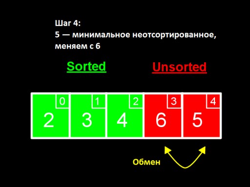 When only one number remains among the unsorted ones (the largest), this means that the entire array is sorted!
 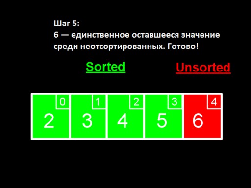 This is what the array implementation looks like in code. Try making it yourself.
 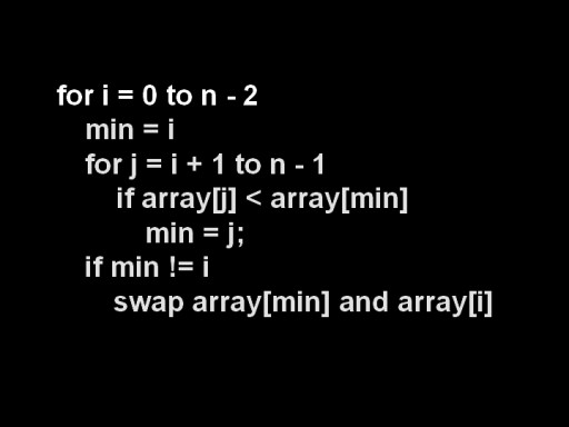 In both the best and worst cases, to find the minimum unsorted element, we must compare each element with each element of the unsorted array, and we will do this at each iteration. But we do not need to view the entire list, but only the unsorted part. Does this change the speed of the algorithm? In the first step, for an array of 5 elements, we make 4 comparisons, in the second - 3, in the third - 2. To get the number of comparisons, we need to add up all these numbers. We get the sum
  Thus, the expected speed of the algorithm in the best and worst cases is Θ(n 2 ). Not the most efficient algorithm! However, for educational purposes and for small data sets it is quite applicable.
 Step 1: go through the array. The algorithm starts with the first two elements, 8 and 6, and checks to see if they are in the correct order. 8 > 6, so we swap them. Next we look at the second and third elements, now these are 8 and 4. For the same reasons, we swap them. For the third time we compare 8 and 2. In total, we make three exchanges (8, 6), (8, 4), (8, 2). The value 8 "floated" to the end of the list in the correct position.
  Step 2: swap (6,4) and (6,2). 6 is now in the penultimate position, and there is no need to compare it with the already sorted “tail” of the list.
  Step 3: swap 4 and 2. The four “floats up” to its rightful place.
  Step 4: we go through the array, but we have nothing to change. This signals that the array is completely sorted.
 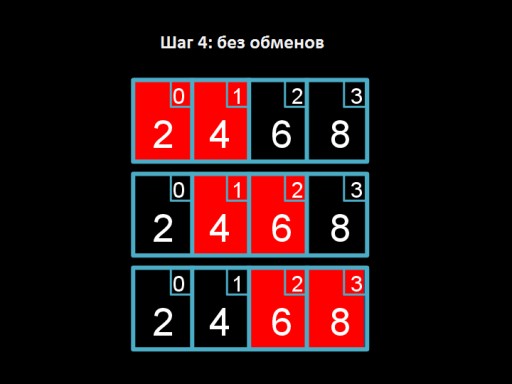 And this is the algorithm code. Try implementing it in C!
  Bubble sort takes O(n 2 ) time in the worst case (all numbers are wrong), since we need to take n steps at each iteration, of which there are also n. In fact, as in the case of the selection sort algorithm, the time will be slightly less (n 2 /2 – n/2), but this can be neglected. In the best case (if all the elements are already in place), we can do it in n steps, i.e. Ω(n), since we will just need to iterate through the array once and make sure that all the elements are in place (i.e. even n-1 elements).
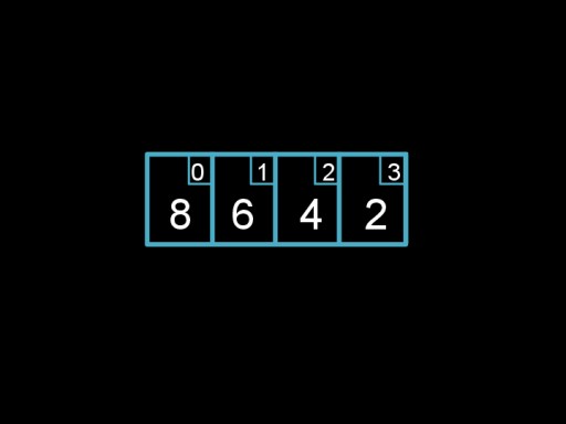
 Let's look at how insertion sort works using the example below. Before we start, all elements are considered unsorted.
  Step 1: Take the first unsorted value (3) and insert it into the sorted subarray. At this step, the entire sorted subarray, its beginning and end will be this very three.
  Step 2: Since 3 > 5, we will insert 5 into the sorted subarray to the right of 3.
  Step 3: Now we work on inserting the number 2 into our sorted array. We compare 2 with values from right to left to find the correct position. Since 2 < 5 and 2 < 3 and we have reached the beginning of the sorted subarray. Therefore, we must insert 2 to the left of 3. To do this, move 3 and 5 to the right so that there is room for the 2 and insert it at the beginning of the array.
  Step 4. We're lucky: 6 > 5, so we can insert that number right after the number 5.
  Step 5. 4 < 6 and 4 < 5, but 4 > 3. Therefore, we know that 4 must be inserted to the right of 3. Again, we are forced to move 5 and 6 to the right to create a gap for 4.
  Done! Generalized Algorithm: Take each unsorted element of n and compare it with the values in the sorted subarray from right to left until we find a suitable position for n (that is, the moment we find the first number that is less than n). Then we shift all the sorted elements that are to the right of this number to the right to make room for our n, and we insert it there, thereby expanding the sorted part of the array. For each unsorted element n you need:
 Let's say we have n elements to sort. If n < 2, we finish sorting, otherwise we sort the left and right parts of the array separately, and then combine them. Let's sort the array.
 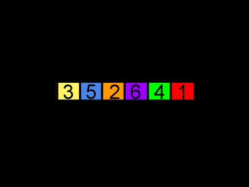 Divide it into two parts, and continue dividing until we get subarrays of size 1, which are obviously sorted.
  Two sorted subarrays can be merged in O(n) time using a simple algorithm: remove the smaller number at the beginning of each subarray and insert it into the merged array. Repeat until all the elements are gone.
 Merge sort takes O(nlog n) time for all cases. While we are dividing the arrays into halves at each recursion level we get log n. Then, merging the subarrays requires only n comparisons. Therefore O(nlog n). The best and worst cases for merge sort are the same, the expected running time of the algorithm = Θ(nlog n). This algorithm is the most effective among those considered.

GO TO FULL VERSION